Inno-QSAR
1. Overview of Inno-QSAR
Quantitative Structure–Activity Relationship (QSAR) is a methodological approach that studies the relationship between the chemical structure and physicochemical properties of compounds and their biological activities, thereby establishing quantitative (or qualitative) predictive models. With the rapid development of computer technology, QSAR modeling based on various machine learning (ML) algorithms has emerged. ML and deep learning (DL) methods such as Random Forest (RF) and eXtreme Gradient Boosting (XGBoost) have gradually replaced the original Hansch and Free-Wilson methods. By employing these algorithms to learn from the known biological activities of compounds and their corresponding structures or physicochemical properties, one can build a QSAR classification or regression model, thus effectively distinguishing active from inactive molecules or predicting the biological activity of new compounds.
The most critical factor for a model is its performance, which is mainly affected by three elements: dataset, descriptors, and algorithms.
Dataset: The dataset is the cornerstone of a model; it directly determines the final reliability and practical value of the model. A dataset with more structural diversity and quantity allows for a broader application domain and greater utility. Therefore, users should collect as much data as possible before modeling.
Descriptors (optional, only for ML algorithms): Descriptors offer a more complex representation of molecules, assigned as particular values for specific features, rather than simple binary coding like molecular fingerprints. When building a model, users should select suitable descriptors according to their research purpose to represent relevant molecular information.
Algorithms: ML/DL-based algorithms have significant advantages over traditional approaches but also involve numerous parameters that are difficult to tune. Multiple rounds of tuning are usually required to achieve a high-performing model. To address this, we have simplified the parameter tuning process by exposing only a few key parameters and providing default values, enabling users to easily build high-quality QSAR models.
The Inno-QSAR module enables rapid AI modeling using your own data, supporting mainstream data cleaning, dataset splitting, descriptor calculation, and ML/DL algorithm selection. Users can choose an automatic modeling mode or manually adjust the parameters for optimal performance. The result page provides comprehensive model evaluation and statistical charting functionality. The constructed models can be conveniently integrated into system workflows.
2. User Guide
Users can complete the calculation in six steps: select model type – upload data – set modeling data – set modeling method – name the task (optional) – submit task (required).
(1) Select Model Type
Users should select the desired model type according to their needs: classification model or regression model.
(2) Upload Data
Uploading data includes both training and test sets.
The platform provides two methods for data input: uploading files or selecting from the data center.
- Upload File
Check the "Upload File" box and click the button below to select a local file. The contents of the selected file will then be displayed on the right.
- Supported file formats: .sdf/.csv
- Data Center
Check the "Data Center" box, click the button below, and a popup window will appear. Select data from the data center by clicking the file name. The popup will close after selection.

Figure 1. Data input: upload file/data center
- Test Set
- If you have already saved the training and test sets as separate files, upload each one accordingly.
- If you have not pre-divided your data, you can upload a file for the training set only and turn off the switch behind the test set. The test set will be automatically split according to your specified ratio and sampling method. As shown in Figure 2, 10% of the data will be extracted from the training set as the test set.
After preprocessing, the statistical distributions of the training and test sets will be plotted, helping users quickly understand the distribution of the actual data to be modeled. Detailed model parameters are also displayed on this page.

Figure 2. Automatic splitting of test set
(3) Set Modeling Data
SMILES column – specify the SMILES column.
Label column – specify the label/target column.
Active value – for classification models, specify which label value represents activity.
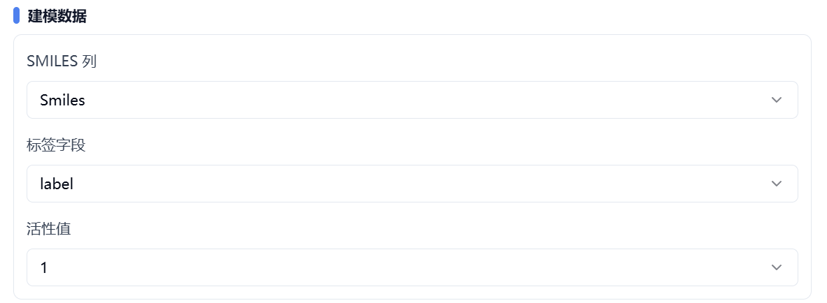
Figure 3. Set modeling data
(4) Set Modeling Method
The platform provides two main categories of modeling methods: descriptor-based and structure-based. Descriptor-based algorithms include AutoML, XGBoost, and RF. Structure-based algorithms include Transformer (Pretrain) and GNN (Pretrain).
- Descriptor-Based
Descriptor-based methods are for machine learning models. First, select one algorithm from AutoML, RF, or XGBoost. Next, set up descriptors. The platform provides two ways: compute new descriptors or user-defined.
- Compute New Descriptors
Users can select one or more descriptor types from ECFP4, ECFP6, MACCS, and MoleculeDescriptors. The platform will automatically calculate the selected descriptors.
ECFP4/6: ECFP (Extended-Connectivity Fingerprints) are circular fingerprints that contain highly specific atomic information for representing substructure features. The number specifies the maximum diameter of the circle considered for each atom. The default diameter is 4, suitable for similarity searching and clustering, while 6/8 is better for larger structural fragments and activity prediction.
MACCS: MACCS descriptors are structural descriptors containing 166 common substructure features.
MoleculeDescriptors: These refer to the 115 2D descriptors provided in RDKit.
- User-Defined
Users can pre-calculate the descriptors and save them in the uploaded file, then specify the columns containing these descriptors here.
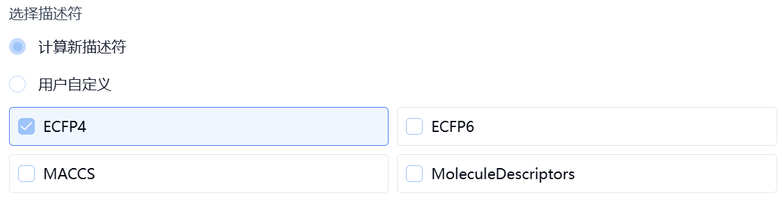
Figure 4. Set modeling method – compute descriptors
- Structure-Based
Structure-based methods are mainly aimed at deep learning algorithms. First, select one algorithm from Transformer (Pretrain) or GNN (Pretrain). Both algorithms have been pre-trained on large-scale datasets.
Next, set the values for num_train_epochs, batch_size, and learning_rate.
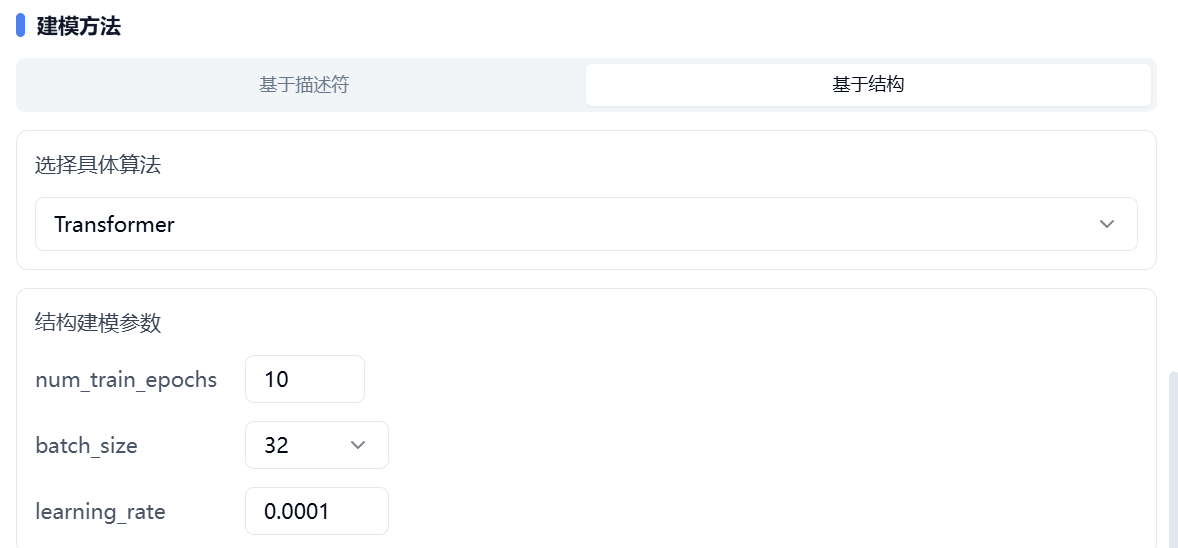
Figure 5. Set modeling method – structure-based
After confirming all parameters, name the task and click "Submit" to complete the submission.
(5) Task Progress and Result Viewing
After submitting the task, the page will automatically jump to the "Recent Results" tab, where you can check the running status (progress bar) of current module tasks. You can also check all running tasks from different modules via the "Notifications" dropdown in the upper-right corner. Once the task has finished, click "View Results" to visit the results page and view the finished results.

Figure 6. View results
3. Results Analysis
The results page is divided into two main sections: Training Results and Data Distribution.
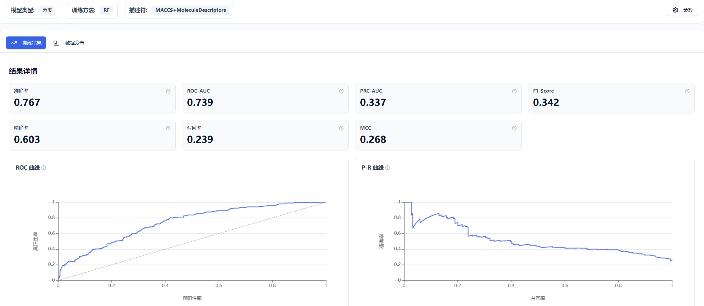
Figure 7. Inno-QSAR result page layout
(1) Training Results
- Classification Models
For classification models, performance metrics are computed based on the test set, including Accuracy, ROC-AUC, PRC-AUC, F1-Score, Precision, Recall, and MCC. The ROC curve and P-R curve are also provided.
- Regression Models
For regression models, metrics computed based on the test set include MAE, MSE, RMSE, R2, and PCCs, along with a scatter plot showing the correlation between true and predicted values.
(2) Data Distribution
4. Algorithm Introduction
(1) AutoML
AutoML contains 11 algorithms. Based on the user's input data, it automates processes such as handling missing data, manual feature transformation, data splitting, model selection, algorithm selection, hyperparameter selection and tuning, and ensemble modeling, replacing traditionally time-consuming manual steps. By using L-layer stacking and n-repeated k-bagging ensembling techniques, it not only accelerates computation but also greatly improves model accuracy. AutoML will automatically filter out unsuitable models based on the input data, weight the results of successfully built models, and finally output a weighted average of those models.
The 11 algorithms referenced above include:
(2) XGBoost
XGBoost is a machine learning algorithm based on ensemble learning that primarily uses gradient boosting to build an ensemble model. By iteratively adding weak learners, XGBoost improves upon the residuals in each iteration. It also uses regularization to control model complexity and avoids overfitting. During training, the platform uses a combination of grid search and 5-fold cross-validation to identify optimal parameters, thereby enhancing model accuracy and generalization ability, and mitigating performance bias due to uneven data distribution.
(3) RF (Random Forest)
Random Forest is an ensemble algorithm based on decision trees. It builds multiple decision trees by bootstrapping the dataset (sampling with replacement) and randomly selecting features for each sample in each tree. The final prediction is the combination (by voting or averaging) of all trees. RF can effectively handle high-dimensional data and nonlinear relationships, and also reduces the risk of overfitting. During training, the platform uses a combination of grid search and 5-fold cross-validation to select optimal parameters and improve model generalization and accuracy, while avoiding performance bias from uneven data distribution.
(4) Transformer (Pretrain)
Transformer (Pretrain) is a proprietary pre-trained model developed by Carbon Silicon Intelligence. It utilizes 3.3 million small molecule data entries, taking 1D, 2D, and 3D molecular information as input. It adopts the philosophy of "alignment before fusion" of modalities, leveraging Contrast Loss, Matching Loss, and Momentum Encoder strategies to constrain global molecular features. The homo-lumo gap is used as a supervised signal to restrict molecular physical properties. The model employs a 3D molecular conformation denoising task to regularize 3D structure, and introduces a molecular fragment localization auxiliary task to focus on local molecular information. The MOE (Mixture-of-Experts) architecture significantly enhances the model's multi-modal adaptability. Evaluation across multiple datasets shows a clear improvement in modeling performance especially on small datasets.
(5) GNN (Pretrain)
GNN (Pretrain) is a proprietary pre-trained model developed by Carbon Silicon Intelligence. It encodes molecular graphs using atomic and bond features (including 9 types of atomic features and 5 types of bond features for atoms, bonds, and their local environments), extracting general features from substructures via several shared-parameter RGCN layers, and applies attention layers to assign different attention weights to substructures, resulting in a high-performance pre-trained model. Its benefits are: (1) Regularization – the model can learn more tasks with the same number of parameters; (2) Transfer learning – since ADMET data are correlated, sharing parameters in certain hidden layers among related tasks helps extract general features; (3) Data augmentation – as ADMET data are sparse, training on all the tasks simultaneously prevents overfitting on small tasks.
5. References
None currently available.